3.1 Gallery 
This gallery collects the example plots generated from the scripts in docs/scripts. Each subsection includes a brief description, the generated image, and the full script source.
- Bessel Functions
- Chebyshev Polynomials
- Damped Harmonic Oscillator
- Elliptic-Integral Pendulum Period
- Fourier Series Approximation
- Cornu Spiral from Fresnel Integrals
- Gamma Function
- Gaussian Density Curves
- Lissajous Figures
- Lotka-Volterra Dynamics
- Logistic Map Orbit Diagram
- Prime Counting and Logarithmic Integral
- Weierstrass Function
- Riemann Zeta on the Real Line
- Dragon Curve
- Gaussian Histogram
- Golden Spiral
- Hilbert Curve
- Koch Snowflake
- Sierpinski Triangle
- Spirograph Curves
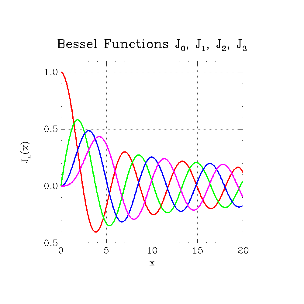
3.1.1 Bessel Functions 
This plot shows the Bessel functions of the first kind J_n(x) for several low orders. These functions arise naturally in cylindrical wave and diffusion problems.
;;; ex-graph-bessel.scm — Bessel functions of the first kind J_n(x)
;;; J_n(x) = Σ_{m=0}^{∞} (−1)^m / (m! · Γ(m+n+1)) · (x/2)^(2m+n)
;;; Bessel functions arise as solutions to Laplace's equation in
;;; cylindrical coordinates—fundamental to acoustics of drums, heat
;;; conduction in cylinders, and electromagnetic waveguides.

(use-modules (srfi srfi-1)
             (plotutils graph))

(define (factorial n)
  (if (<= n 1) 1
      (let loop ((i 2) (acc 1))
        (if (> i n) acc
            (loop (+ i 1) (* acc i))))))

(define (bessel-j order x)
  "Compute J_order(x) via power series, for non-negative integer order."
  (let ((terms 25))
    (let loop ((m 0) (acc 0.0))
      (if (> m terms)
          acc
          (let* ((sign (if (even? m) 1.0 -1.0))
                 (num (expt (/ x 2.0) (+ (* 2 m) order)))
                 (den (* (factorial m) (factorial (+ m order)))))
            (loop (+ m 1) (+ acc (/ (* sign num) den))))))))

(define (output-format-from-filename path)
  (let loop ((i (- (string-length path) 1)))
    (cond
     ((< i 0) "svg")
     ((char=? (string-ref path i) #\.)
      (let ((ext (string-downcase (substring path (+ i 1) (string-length path)))))
        (if (string=? ext "eps") "ps" ext)))
     (else (loop (- i 1))))))

(define (main args)
  (let* ((output-file (if (> (length args) 1) (cadr args) "graph-bessel.svg"))
         (output-format (output-format-from-filename output-file))
         (n 500)
         (xmin 0.0)
         (xmax 20.0)
         (step (/ (- xmax xmin) n))
         (xs (iota n xmin step))
         (j0 (map (lambda (x) (bessel-j 0 x)) xs))
         (j1 (map (lambda (x) (bessel-j 1 x)) xs))
         (j2 (map (lambda (x) (bessel-j 2 x)) xs))
         (j3 (map (lambda (x) (bessel-j 3 x)) xs)))
    (with-output-to-file output-file
      (lambda ()
        (graph (merge xs xs xs xs)
               (merge j0 j1 j2 j3)
               #:output-format output-format
               #:bitmap-size "1000x1000"
               #:top-label "Bessel Functions J\\sb0\\eb, J\\sb1\\eb, J\\sb2\\eb, J\\sb3\\eb"
               #:x-label "x"
               #:y-label "J\\sbn\\eb(x)"
               #:x-limits '(0.0 20.0)
               #:y-limits '(-0.5 1.1)
               #:toggle-use-color #t
               #:grid-style 3
               #:line-width 0.004
               #:font-name "HersheySerif"))
      #:binary #t)))
(main (command-line))
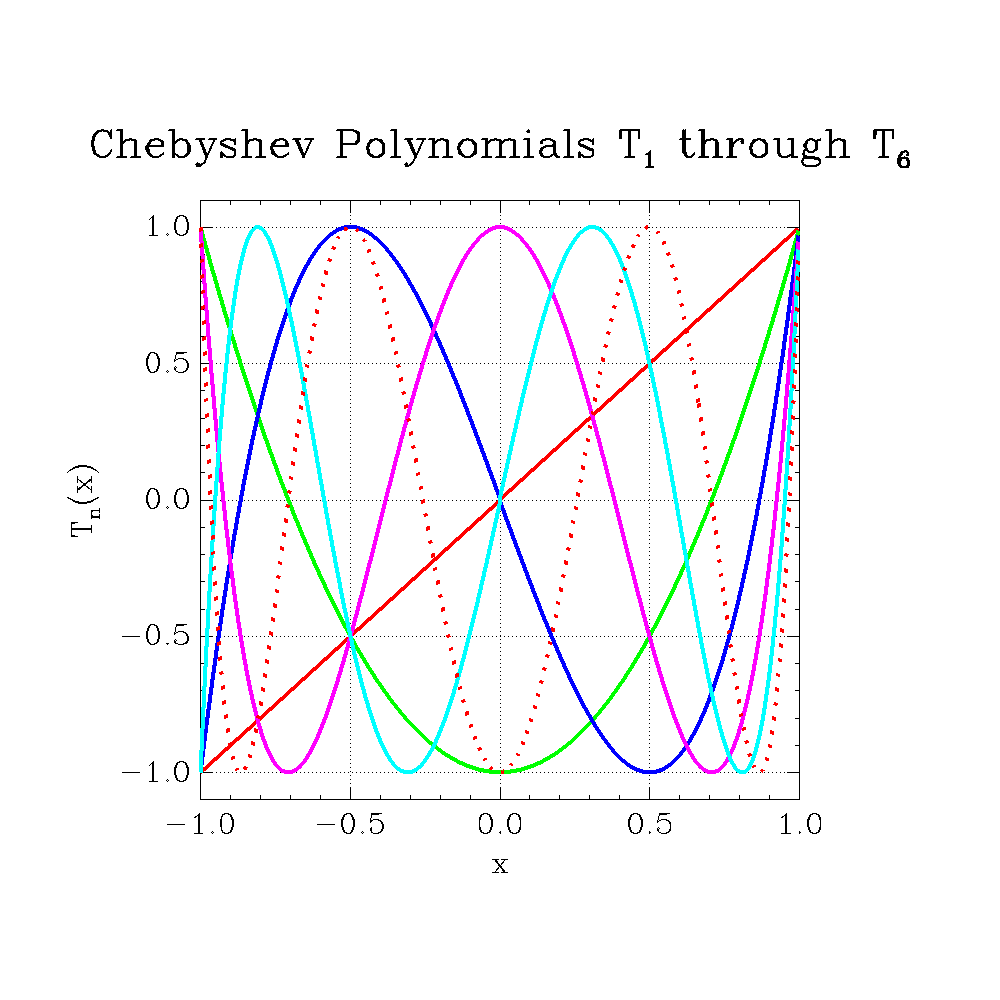
3.1.2 Chebyshev Polynomials 
This plot draws Chebyshev polynomials Tn(x), a classical family of orthogonal polynomials used heavily in approximation theory and spectral methods.
;;; ex-graph-chebyshev.scm — Chebyshev polynomials of the first kind T_n(x)
;;; T_0(x) = 1,  T_1(x) = x,  T_{n+1}(x) = 2x·T_n(x) − T_{n−1}(x)
;;; Chebyshev polynomials are orthogonal on [−1,1] w.r.t. the weight
;;; 1/√(1−x²), minimize the maximum deviation among polynomials of the
;;; same degree (minimax property), and are the backbone of spectral
;;; methods for numerical PDEs and optimal polynomial interpolation.

(use-modules (srfi srfi-1)
             (plotutils graph))

(define (chebyshev n x)
  "Compute T_n(x) via the three-term recurrence."
  (cond
   ((= n 0) 1.0)
   ((= n 1) x)
   (else
    (let loop ((k 2) (t-prev 1.0) (t-curr x))
      (let ((t-next (- (* 2.0 x t-curr) t-prev)))
        (if (= k n)
            t-next
            (loop (+ k 1) t-curr t-next)))))))

(define (output-format-from-filename path)
  (let loop ((i (- (string-length path) 1)))
    (cond
     ((< i 0) "svg")
     ((char=? (string-ref path i) #\.)
      (let ((ext (string-downcase (substring path (+ i 1) (string-length path)))))
        (if (string=? ext "eps") "ps" ext)))
     (else (loop (- i 1))))))

(define (main args)
  (let* ((output-file (if (> (length args) 1) (cadr args) "graph-chebyshev.svg"))
         (output-format (output-format-from-filename output-file))
         (n 600)
         (xmin -1.0)
         (xmax 1.0)
         (step (/ (- xmax xmin) n))
         (xs (iota n xmin step))
         (t1 (map (lambda (x) (chebyshev 1 x)) xs))
         (t2 (map (lambda (x) (chebyshev 2 x)) xs))
         (t3 (map (lambda (x) (chebyshev 3 x)) xs))
         (t4 (map (lambda (x) (chebyshev 4 x)) xs))
         (t5 (map (lambda (x) (chebyshev 5 x)) xs))
         (t6 (map (lambda (x) (chebyshev 6 x)) xs)))
    (with-output-to-file output-file
      (lambda ()
        (graph (merge xs xs xs xs xs xs)
               (merge t1 t2 t3 t4 t5 t6)
               #:output-format output-format
               #:bitmap-size "1000x1000"
               #:top-label "Chebyshev Polynomials T\\sb1\\eb through T\\sb6\\eb"
               #:x-label "x"
               #:y-label "T\\sbn\\eb(x)"
               #:x-limits '(-1.0 1.0)
               #:y-limits '(-1.1 1.1)
               #:toggle-use-color #t
               #:grid-style 3
               #:line-width 0.004
               #:font-name "HersheySerif"))
      #:binary #t)))

(main (command-line))
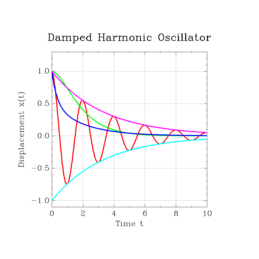
3.1.3 Damped Harmonic Oscillator 
This plot illustrates damped oscillatory behavior, covering underdamped, critical, and overdamped regimes for a mass-spring-damper model.
;;; ex-graph-damped-oscillator.scm — Damped harmonic oscillator
;;; x(t) = A·e^(−γt)·cos(ωt − φ)
;;; The fundamental solution to the second-order ODE of a mass-spring-damper
;;; system.  Shows underdamped, critically damped, and overdamped regimes.

(use-modules (srfi srfi-1)
             (plotutils graph))

(define pi (* 4.0 (atan 1.0)))

(define (underdamped gamma omega)
  (lambda (t)
    (* (exp (* (- gamma) t)) (cos (* omega t)))))

(define (critically-damped gamma)
  (lambda (t)
    (* (+ 1.0 (* gamma t)) (exp (* (- gamma) t)))))

(define (overdamped r1 r2)
  "Overdamped: x(t) = A·e^(r1·t) + B·e^(r2·t), both r1,r2 < 0."
  (lambda (t)
    (+ (* 0.5 (exp (* r1 t)))
       (* 0.5 (exp (* r2 t))))))

(define (output-format-from-filename path)
  (let loop ((i (- (string-length path) 1)))
    (cond
     ((< i 0) "svg")
     ((char=? (string-ref path i) #\.)
      (let ((ext (string-downcase (substring path (+ i 1) (string-length path)))))
        (if (string=? ext "eps") "ps" ext)))
     (else (loop (- i 1))))))

(define (main args)
  (let* ((output-file (if (> (length args) 1) (cadr args) "graph-damped-oscillator.svg"))
         (output-format (output-format-from-filename output-file))
         (n 500)
         (tmin 0.0)
         (tmax 10.0)
         (step (/ (- tmax tmin) n))
         (ts (iota n tmin step))
         ;; Underdamped: γ=0.3, ω=2π·0.5
         (y-under (map (underdamped 0.3 (* 2.0 pi 0.5)) ts))
         ;; Critically damped: γ=1.0
         (y-crit (map (critically-damped 1.0) ts))
         ;; Overdamped: roots r1=-0.5, r2=-3.0
         (y-over (map (overdamped -0.5 -3.0) ts))
         ;; Envelope for underdamped
         (y-env+ (map (lambda (t) (exp (* -0.3 t))) ts))
         (y-env- (map (lambda (t) (- (exp (* -0.3 t)))) ts)))
    (with-output-to-file output-file
      (lambda ()
        (graph (merge ts ts ts ts ts)
               (merge y-under y-crit y-over y-env+ y-env-)
               #:output-format output-format
               #:bitmap-size "1000x1000"
               #:top-label "Damped Harmonic Oscillator"
               #:x-label "Time t"
               #:y-label "Displacement x(t)"
               #:x-limits '(0.0 10.0)
               #:y-limits '(-1.1 1.3)
               #:toggle-use-color #t
               #:grid-style 3
               #:line-width 0.004
               #:font-name "HersheySerif"))
      #:binary #t)))

(main (command-line))
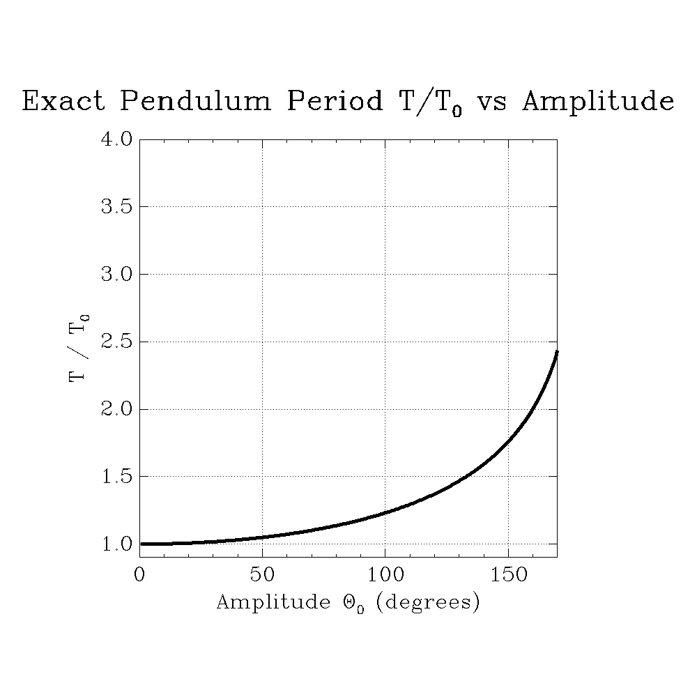
3.1.4 Elliptic-Integral Pendulum Period 
This plot shows the exact pendulum period ratio as amplitude increases, using the complete elliptic integral of the first kind.
;;; ex-graph-elliptic-integral.scm — Complete elliptic integrals K(k) and E(k)
;;; K(k) = ∫₀^{π/2} dθ / √(1 − k²sin²θ)   (first kind)
;;; E(k) = ∫₀^{π/2} √(1 − k²sin²θ) dθ      (second kind)
;;; These arise in computing arc lengths of ellipses, pendulum periods
;;; (K appears in the exact period of a simple pendulum), and in the
;;; theory of elliptic curves central to modern number theory and cryptography.
;;; K(k) → ∞ as k → 1, while E(1) = 1.

(use-modules (srfi srfi-1)
             (plotutils graph))

(define pi (* 4.0 (atan 1.0)))

(define (integrate-simpson f a b n)
  "Numerical integration of f from a to b using Simpson's rule with n subintervals."
  (let* ((h (/ (- b a) n))
         (sum (+ (f a) (f b))))
    (let loop ((i 1) (s sum))
      (if (>= i n)
          (* (/ h 3.0) s)
          (let* ((x (+ a (* i h)))
                 (w (if (even? i) 2.0 4.0)))
            (loop (+ i 1) (+ s (* w (f x)))))))))

(define (elliptic-k k)
  "Complete elliptic integral of the first kind."
  (integrate-simpson
   (lambda (theta) (/ 1.0 (sqrt (- 1.0 (* k k (sin theta) (sin theta))))))
   0.0 (- (/ pi 2.0) 1e-10) 500))

(define (elliptic-e k)
  "Complete elliptic integral of the second kind."
  (integrate-simpson
   (lambda (theta) (sqrt (- 1.0 (* k k (sin theta) (sin theta)))))
   0.0 (/ pi 2.0) 500))

(define (output-format-from-filename path)
  (let loop ((i (- (string-length path) 1)))
    (cond
     ((< i 0) "svg")
     ((char=? (string-ref path i) #\.)
      (let ((ext (string-downcase (substring path (+ i 1) (string-length path)))))
        (if (string=? ext "eps") "ps" ext)))
     (else (loop (- i 1))))))

(define (main args)
  (let* ((output-file (if (> (length args) 1) (cadr args) "graph-pendulum-period.svg"))
         (output-format (output-format-from-filename output-file))
         ;; Exact pendulum period T/T_0 = (2/π)K(k) where k = sin(θ_0/2)
         ;; Show for θ_0 from 0 to ~170°
         (n2 300)
         (theta-max (* 170.0 (/ pi 180.0)))
         (theta-step (/ theta-max n2))
         (thetas (iota n2 0.01 theta-step))
         (theta-deg (map (lambda (t) (* t (/ 180.0 pi))) thetas))
         (period-ratio (map (lambda (t)
                              (* (/ 2.0 pi) (elliptic-k (sin (/ t 2.0)))))
                            thetas)))
    ;; Exact pendulum period ratio
    (with-output-to-file output-file
      (lambda ()
        (graph theta-deg period-ratio
               #:output-format output-format
               #:bitmap-size "1000x1000"
               #:top-label "Exact Pendulum Period T/T\\sb0\\eb vs Amplitude"
               #:x-label "Amplitude \\*H\\sb0\\eb (degrees)"
               #:y-label "T / T\\sb0\\eb"
               #:x-limits '(0.0 170.0)
               #:y-limits '(0.9 4.0)
               #:grid-style 3
               #:line-width 0.005
               #:font-name "HersheySerif"))
      #:binary #t)))

(main (command-line))
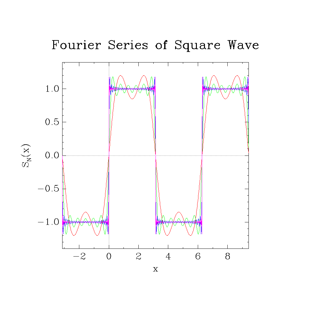
3.1.5 Fourier Series Approximation 
This plot visualizes partial sums of a Fourier series approximation to a square wave, including the Gibbs overshoot near jump discontinuities.
;;; ex-graph-fourier.scm — Fourier series approximation of a square wave
;;; Demonstrates Gibbs phenomenon: partial sums of the Fourier series
;;; overshoot near the discontinuity by ~9%, no matter how many terms.
;;; S_N(x) = (4/π) Σ_{k=0}^{N} sin((2k+1)x) / (2k+1)

(use-modules (srfi srfi-1)
             (plotutils graph))

(define pi (* 4.0 (atan 1.0)))

(define (fourier-square-wave n-terms)
  "Return a procedure computing the N-term Fourier partial sum of a square wave."
  (lambda (x)
    (let loop ((k 0) (acc 0.0))
      (if (> k n-terms)
          acc
          (let ((m (+ (* 2 k) 1)))
            (loop (+ k 1)
                  (+ acc (* (/ 4.0 pi) (/ (sin (* m x)) m)))))))))

(define (output-format-from-filename path)
  (let loop ((i (- (string-length path) 1)))
    (cond
     ((< i 0) "svg")
     ((char=? (string-ref path i) #\.)
      (let ((ext (string-downcase (substring path (+ i 1) (string-length path)))))
        (if (string=? ext "eps") "ps" ext)))
     (else (loop (- i 1))))))

(define (main args)
  (let* ((output-file (if (> (length args) 1) (cadr args) "graph-fourier.svg"))
         (output-format (output-format-from-filename output-file))
         (n 800)
         (xmin (- pi))
         (xmax (* 3 pi))
         (step (/ (- xmax xmin) n))
         (xs (iota n xmin step))
         (y1 (map (fourier-square-wave 1) xs))
         (y2 (map (fourier-square-wave 5) xs))
         (y3 (map (fourier-square-wave 25) xs))
         (y4 (map (fourier-square-wave 100) xs)))
    (with-output-to-file output-file
      (lambda ()
        (graph (merge xs xs xs xs)
               (merge y1 y2 y3 y4)
               #:output-format output-format
               #:bitmap-size "1000x1000"
               #:top-label "Fourier Series of Square Wave"
               #:x-label "x"
               #:y-label "S\\sbN\\eb(x)"
               #:x-limits (list (- pi) (* 3 pi))
               #:y-limits '(-1.4 1.4)
               #:toggle-use-color #t
               #:grid-style 2
               #:font-name "HersheySerif"))
      #:binary #t)))

(main (command-line))
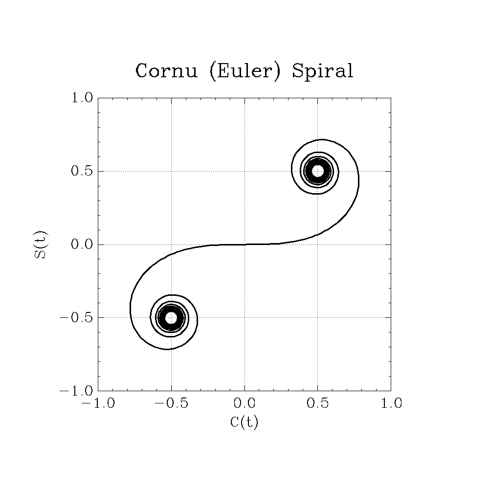
3.1.6 Cornu Spiral from Fresnel Integrals 
This plot draws the Cornu (Euler) spiral, parameterized by Fresnel integrals, a central curve in diffraction theory.
;;; ex-graph-fresnel.scm — Fresnel integrals S(x) and C(x)
;;; S(x) = ∫₀ˣ sin(π/2·t²) dt,  C(x) = ∫₀ˣ cos(π/2·t²) dt
;;; These arise in diffraction theory (Fresnel diffraction at a straight
;;; edge).  Both oscillate and converge to ½ as x → ∞.  Also plots the
;;; Cornu (Euler) spiral: the parametric curve (C(t), S(t)).

(use-modules (srfi srfi-1)
             (plotutils graph))

(define pi (* 4.0 (atan 1.0)))

(define (integrate-simpson f a b n)
  "Numerical integration of f from a to b using Simpson's rule
with n subintervals."
  (let* ((h (/ (- b a) n))
         (sum (+ (f a) (f b))))
    (let loop ((i 1) (s sum))
      (if (>= i n)
          (* (/ h 3.0) s)
          (let* ((x (+ a (* i h)))
                 (w (if (even? i) 2.0 4.0)))
            (loop (+ i 1) (+ s (* w (f x)))))))))

(define (fresnel-s x)
  (if (= x 0.0) 0.0
      (integrate-simpson (lambda (t) (sin (* (/ pi 2.0) t t)))
                         0.0 x 200)))

(define (fresnel-c x)
  (if (= x 0.0) 0.0
      (integrate-simpson (lambda (t) (cos (* (/ pi 2.0) t t)))
                         0.0 x 200)))

(define (output-format-from-filename path)
  (let loop ((i (- (string-length path) 1)))
    (cond
     ((< i 0) "svg")
     ((char=? (string-ref path i) #\.)
      (let ((ext (string-downcase (substring path (+ i 1) (string-length path)))))
        (if (string=? ext "eps") "ps" ext)))
     (else (loop (- i 1))))))

(define (main args)
  (let* ((output-file (if (> (length args) 1) (cadr args) "graph-cornu-spiral.svg"))
         (output-format (output-format-from-filename output-file))
         ;; Cornu spiral: parametric (C(t), S(t)) for t in [-7, 7]
         (nt 600)
         (tmin -7.0)
         (tmax 7.0)
         (tstep (/ (- tmax tmin) nt))
         (ts (iota nt tmin tstep))
         (spiral-x (map fresnel-c ts))
         (spiral-y (map fresnel-s ts)))
    ;; Cornu (Euler) spiral
    (with-output-to-file output-file
      (lambda ()
        (graph spiral-x spiral-y
               #:output-format output-format
               #:bitmap-size "1000x1000"
               #:top-label "Cornu (Euler) Spiral"
               #:x-label "C(t)"
               #:y-label "S(t)"
               #:x-limits '(-1.0 1.0)
               #:y-limits '(-1.0 1.0)
               #:grid-style 3
               #:line-width 0.003
               #:font-name "HersheySerif"))
      #:binary #t)))

(main (command-line))
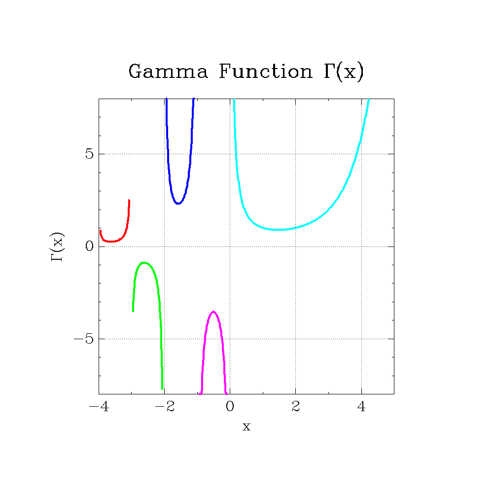
3.1.7 Gamma Function 
This plot shows the Gamma function Gamma(x) on the real line, including behavior near poles at non-positive integers.
;;; ex-graph-gamma.scm — The Gamma function Γ(x) via Lanczos approximation
;;; Γ extends the factorial to real numbers: Γ(n) = (n−1)! for positive
;;; integers.  Has poles at non-positive integers.  Plotted in two
;;; segments avoiding the pole at x=0.

(use-modules (srfi srfi-1)
             (plotutils graph))

(define pi (* 4.0 (atan 1.0)))

(define (lanczos-gamma x)
  "Compute Γ(x) using the Lanczos approximation (g=7)."
  (let ((p (list 0.99999999999980993
                 676.5203681218851
                 -1259.1392167224028
                 771.32342877765313
                 -176.61502916214059
                 12.507343278686905
                 -0.13857109526572012
                 9.9843695780195716e-6
                 1.5056327351493116e-7)))
    (if (< x 0.5)
        ;; Reflection formula: Γ(x) = π / (sin(πx) · Γ(1−x))
        (/ pi (* (sin (* pi x)) (lanczos-gamma (- 1.0 x))))
        (let* ((x (- x 1.0))
               (g 7)
               (a (car p))
               (ag (let loop ((i 1) (acc a))
                     (if (>= i (length p))
                         acc
                         (loop (+ i 1)
                               (+ acc (/ (list-ref p i) (+ x i)))))))
               (t (+ x g 0.5)))
          (* (sqrt (* 2.0 pi))
             (expt t (+ x 0.5))
             (exp (- t))
             ag)))))

(define (output-format-from-filename path)
  (let loop ((i (- (string-length path) 1)))
    (cond
     ((< i 0) "svg")
     ((char=? (string-ref path i) #\.)
      (let ((ext (string-downcase (substring path (+ i 1) (string-length path)))))
        (if (string=? ext "eps") "ps" ext)))
     (else (loop (- i 1))))))

(define (main args)
  (let* ((output-file (if (> (length args) 1) (cadr args) "graph-gamma.svg"))
         (output-format (output-format-from-filename output-file))
         (n 300)
         ;; Segment from 0.1 to 5.0 (avoiding pole at 0)
         (xs1-min 0.08)
         (xs1-max 5.0)
         (step1 (/ (- xs1-max xs1-min) n))
         (xs1 (iota n xs1-min step1))
         (ys1 (map lanczos-gamma xs1))
         ;; Segment from -3.95 to -0.05 (between poles)
         (xs2-parts
          ;; Three inter-pole segments: (-3.95,-3.05), (-2.95,-2.05), (-1.95,-0.05)
          (append
           (let* ((a -3.95) (b -3.05) (s (/ (- b a) 80)))
             (map (lambda (i) (+ a (* i s))) (iota 80)))
           (list #f)
           (let* ((a -2.95) (b -2.05) (s (/ (- b a) 80)))
             (map (lambda (i) (+ a (* i s))) (iota 80)))
           (list #f)
           (let* ((a -1.95) (b -1.05) (s (/ (- b a) 80)))
             (map (lambda (i) (+ a (* i s))) (iota 80)))
           (list #f)
           (let* ((a -0.95) (b -0.05) (s (/ (- b a) 80)))
             (map (lambda (i) (+ a (* i s))) (iota 80)))))
         (ys2-parts
          (map (lambda (v) (if v (lanczos-gamma v) #f)) xs2-parts))
         ;; Clamp values for display
         (clamp (lambda (v) (if v (max -8.0 (min 8.0 v)) #f)))
         (ys2-clamped (map clamp ys2-parts)))
    (with-output-to-file output-file
      (lambda ()
        (graph (merge xs2-parts xs1)
               (merge ys2-clamped ys1)
               #:output-format output-format
               #:bitmap-size "1000x1000"
               #:top-label "Gamma Function \\*G(x)"
               #:x-label "x"
               #:y-label "\\*G(x)"
               #:x-limits '(-4.0 5.0)
               #:y-limits '(-8.0 8.0)
               #:toggle-use-color #t
               #:grid-style 3
               #:line-width 0.004
               #:font-name "HersheySerif"))
      #:binary #t)))

(main (command-line))
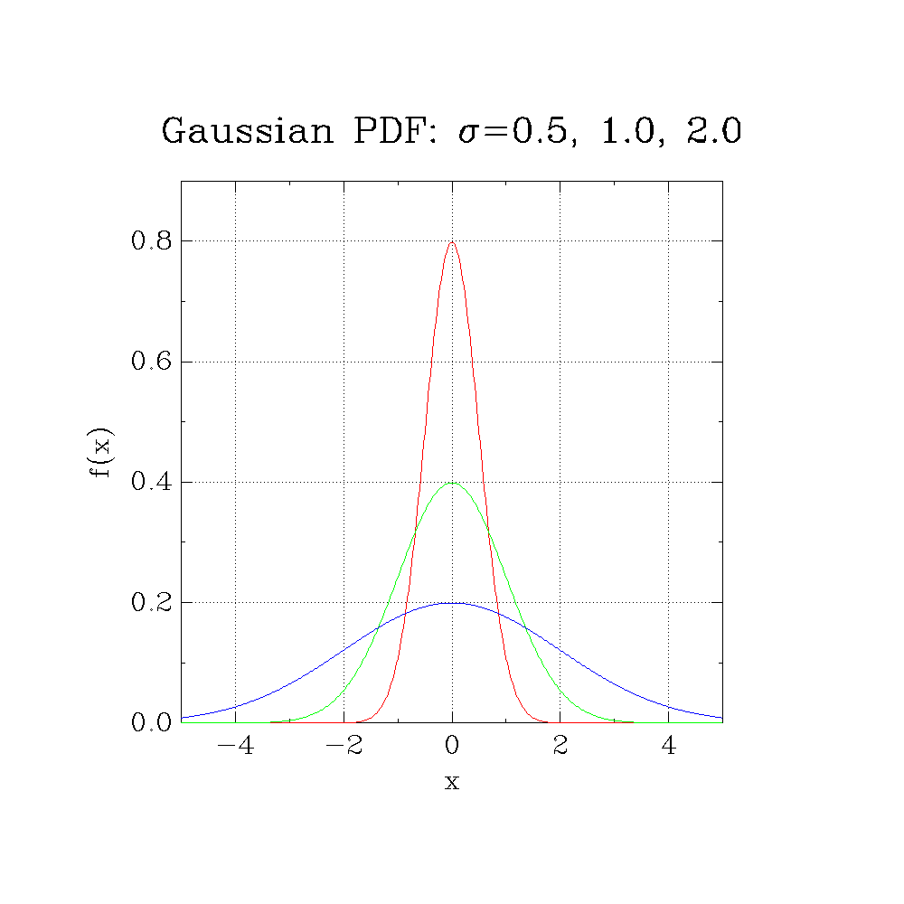
3.1.8 Gaussian Density Curves 
This plot compares Gaussian probability density functions with different standard deviations, emphasizing how variance controls spread.
;;; ex-graph-gaussian.scm — Gaussian (Normal) probability density functions
;;; Plots the bell curve for three different standard deviations,
;;; illustrating how variance controls the spread of a distribution.
;;; f(x) = (1 / (σ√(2π))) · exp(−x²/(2σ²))

(use-modules (srfi srfi-1)
             (plotutils graph))

(define pi (* 4.0 (atan 1.0)))

(define (gaussian sigma)
  (lambda (x)
    (/ (exp (- (/ (* x x) (* 2.0 sigma sigma))))
       (* sigma (sqrt (* 2.0 pi))))))

(define (output-format-from-filename path)
  (let loop ((i (- (string-length path) 1)))
    (cond
     ((< i 0) "svg")
     ((char=? (string-ref path i) #\.)
      (let ((ext (string-downcase (substring path (+ i 1) (string-length path)))))
        (if (string=? ext "eps") "ps" ext)))
     (else (loop (- i 1))))))

(define (main args)
  (let* ((output-file (if (> (length args) 1) (cadr args) "graph-gaussian.svg"))
         (output-format (output-format-from-filename output-file))
         (n 500)
         (xmin -5.0)
         (xmax 5.0)
         (step (/ (- xmax xmin) n))
         (xs (iota n xmin step))
         (y1 (map (gaussian 0.5) xs))
         (y2 (map (gaussian 1.0) xs))
         (y3 (map (gaussian 2.0) xs)))
    (with-output-to-file output-file
      (lambda ()
        (graph (merge xs xs xs)
               (merge y1 y2 y3)
               #:output-format output-format
               #:bitmap-size "1000x1000"
               #:top-label "Gaussian PDF: \\*s=0.5, 1.0, 2.0"
               #:x-label "x"
               #:y-label "f(x)"
               #:x-limits '(-5.0 5.0)
               #:y-limits '(0.0 0.9)
               #:toggle-use-color #t
               #:grid-style 3
               #:font-name "HersheySerif"))
      #:binary #t)))

(main (command-line))
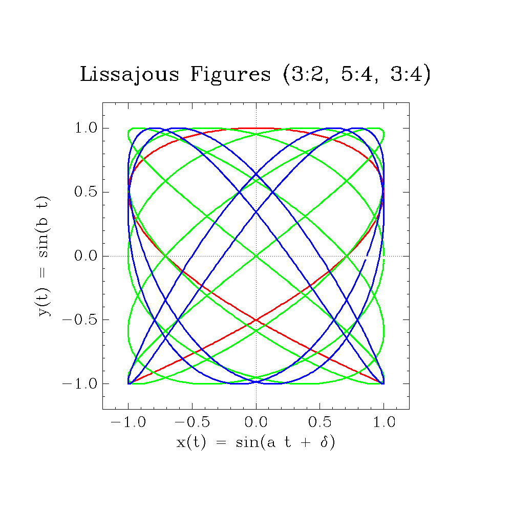
3.1.9 Lissajous Figures 
This plot draws parametric Lissajous curves created by combining two perpendicular harmonic oscillations with different frequency ratios.
;;; ex-graph-lissajous.scm — Lissajous figures (parametric curves)
;;; x(t) = sin(a·t + δ), y(t) = sin(b·t)
;;; These curves arise in physics when two perpendicular harmonic
;;; oscillations are superposed.  The ratio a:b determines the topology.

(use-modules (srfi srfi-1)
             (plotutils graph))

(define pi (* 4.0 (atan 1.0)))

(define (lissajous a b delta n)
  "Return (xlist . ylist) for the Lissajous figure with parameters a, b, delta."
  (let* ((step (/ (* 2.0 pi) n))
         (ts (iota n 0.0 step))
         (xs (map (lambda (t) (sin (+ (* a t) delta))) ts))
         (ys (map (lambda (t) (sin (* b t))) ts)))
    (cons xs ys)))

(define (output-format-from-filename path)
  (let loop ((i (- (string-length path) 1)))
    (cond
     ((< i 0) "svg")
     ((char=? (string-ref path i) #\.)
      (let ((ext (string-downcase (substring path (+ i 1) (string-length path)))))
        (if (string=? ext "eps") "ps" ext)))
     (else (loop (- i 1))))))

(define (main args)
  (let* ((output-file (if (> (length args) 1) (cadr args) "graph-lissajous.svg"))
         (output-format (output-format-from-filename output-file))
         (n 1000)
         (fig1 (lissajous 3 2 (/ pi 4) n))    ; 3:2
         (fig2 (lissajous 5 4 (/ pi 2) n))    ; 5:4
         (fig3 (lissajous 3 4 (/ pi 3) n)))   ; 3:4
    (with-output-to-file output-file
      (lambda ()
        (graph (merge (car fig1) (car fig2) (car fig3))
               (merge (cdr fig1) (cdr fig2) (cdr fig3))
               #:output-format output-format
               #:bitmap-size "1000x1000"
               #:top-label "Lissajous Figures (3:2, 5:4, 3:4)"
               #:x-label "x(t) = sin(a t + \\*d)"
               #:y-label "y(t) = sin(b t)"
               #:x-limits '(-1.2 1.2)
               #:y-limits '(-1.2 1.2)
               #:toggle-use-color #t
               #:grid-style 2
               #:line-width 0.003
               #:font-name "HersheySerif"))
      #:binary #t)))

(main (command-line))
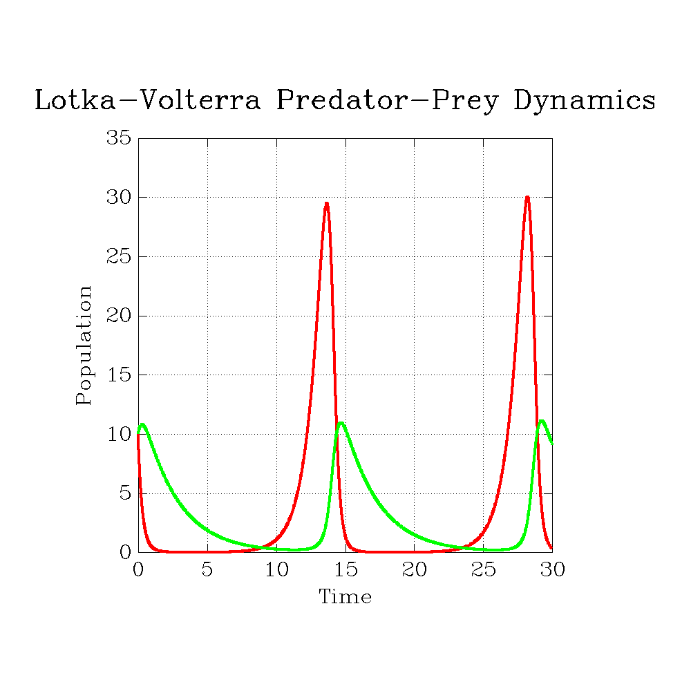
3.1.10 Lotka-Volterra Dynamics 
This plot shows predator-prey oscillations in the Lotka-Volterra model, computed by numerical integration.
;;; ex-graph-logistic-growth.scm — Logistic growth and predator-prey dynamics
;;; 1) Logistic growth: dP/dt = r·P·(1 − P/K), solution P(t) = K/(1 + ((K−P₀)/P₀)e^{−rt})
;;; Models population growth with carrying capacity (Verhulst, 1838).
;;; 2) Lotka-Volterra predator-prey: solved via simple Euler integration,
;;; showing the characteristic oscillatory coexistence cycle.
;;; dx/dt = αx − βxy,  dy/dt = δxy − γy

(use-modules (srfi srfi-1)
             (plotutils graph))

;;; --- Lotka-Volterra via Euler method ---
(define (lotka-volterra alpha beta delta gamma x0 y0 dt n)
  "Return (ts xs ys) for the Lotka-Volterra system."
  (let loop ((i 0) (x x0) (y y0) (ts '()) (xs '()) (ys '()))
    (if (>= i n)
        (list (reverse ts) (reverse xs) (reverse ys))
        (let* ((t (* i dt))
               (dx (* dt (- (* alpha x) (* beta x y))))
               (dy (* dt (- (* delta x y) (* gamma y)))))
          (loop (+ i 1)
                (+ x dx) (+ y dy)
                (cons t ts) (cons x xs) (cons y ys))))))

(define (output-format-from-filename path)
  (let loop ((i (- (string-length path) 1)))
    (cond
     ((< i 0) "svg")
     ((char=? (string-ref path i) #\.)
      (let ((ext (string-downcase (substring path (+ i 1) (string-length path)))))
        (if (string=? ext "eps") "ps" ext)))
     (else (loop (- i 1))))))

(define (main args)
  (let* ((output-file (if (> (length args) 1) (cadr args) "graph-lotka-volterra.svg"))
         (output-format (output-format-from-filename output-file))
         ;; Lotka-Volterra
         (lv (lotka-volterra 1.1 0.4 0.1 0.4 10.0 10.0 0.005 6000))
         (lv-ts (car lv))
         (lv-xs (cadr lv))
         (lv-ys (caddr lv)))
    ;; Lotka-Volterra time series
    (with-output-to-file output-file
      (lambda ()
        (graph (merge lv-ts lv-ts)
               (merge lv-xs lv-ys)
               #:output-format output-format
               #:bitmap-size "1000x1000"
               #:top-label "Lotka-Volterra Predator-Prey Dynamics"
               #:x-label "Time"
               #:y-label "Population"
               #:toggle-use-color #t
               #:grid-style 3
               #:line-width 0.004
               #:font-name "HersheySerif"))
      #:binary #t)))

(main (command-line))
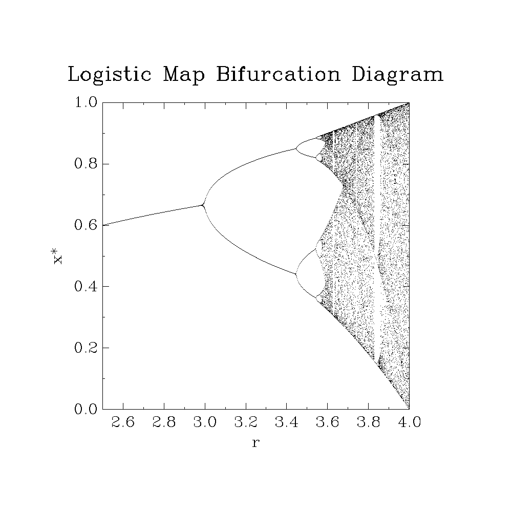
3.1.11 Logistic Map Orbit Diagram 
This plot presents the logistic map bifurcation structure, showing the route from fixed points to period doubling and chaos.
;;; ex-graph-logistic.scm — The Logistic Map orbit diagram
;;; x_{n+1} = r·x_n·(1 − x_n)
;;; For different values of the parameter r, the long-term behavior
;;; transitions from a fixed point to period-doubling cascades to chaos.
;;; This is the canonical example of how simple deterministic systems
;;; produce complex aperiodic dynamics (Feigenbaum universality).

(use-modules (srfi srfi-1)
             (plotutils graph))

(define (logistic-orbit r x0 transient keep)
  "Iterate the logistic map x -> r*x*(1-x) from x0.
Discard TRANSIENT iterates then collect KEEP iterates.
Returns (r-list . x-list) for plotting."
  (let iterate ((i 0) (x x0))
    (if (< i transient)
        (iterate (+ i 1) (* r x (- 1.0 x)))
        ;; Now collect
        (let collect ((j 0) (x x) (rs '()) (xs '()))
          (if (>= j keep)
              (cons (reverse rs) (reverse xs))
              (let ((xnew (* r x (- 1.0 x))))
                (collect (+ j 1) xnew
                         (cons r rs) (cons xnew xs))))))))

(define (output-format-from-filename path)
  (let loop ((i (- (string-length path) 1)))
    (cond
     ((< i 0) "svg")
     ((char=? (string-ref path i) #\.)
      (let ((ext (string-downcase (substring path (+ i 1) (string-length path)))))
        (if (string=? ext "eps") "ps" ext)))
     (else (loop (- i 1))))))

(define (main args)
  (let* ((output-file (if (> (length args) 1) (cadr args) "graph-logistic.svg"))
         (output-format (output-format-from-filename output-file))
         (r-min 2.5)
         (r-max 4.0)
         (n-r 600)
         (r-step (/ (- r-max r-min) n-r))
         (transient 200)
         (keep 80)
         (result
          (let loop ((i 0) (all-r '()) (all-x '()))
            (if (>= i n-r)
                (cons (reverse all-r) (reverse all-x))
                (let* ((r (+ r-min (* i r-step)))
                       (orb (logistic-orbit r 0.4 transient keep)))
                  (loop (+ i 1)
                        (append (car orb) all-r)
                        (append (cdr orb) all-x))))))
         (xs (car result))
         (ys (cdr result)))
    (with-output-to-file output-file
      (lambda ()
        (graph xs ys
               #:output-format output-format
               #:bitmap-size "1000x1000"
               #:top-label "Logistic Map Bifurcation Diagram"
               #:x-label "r"
               #:y-label "x*"
               #:x-limits '(2.5 4.0)
               #:y-limits '(0.0 1.0)
               #:line-mode 0
               #:symbol '(1 0.004)
               #:grid-style 2
               #:font-name "HersheySerif"))
      #:binary #t)))

(main (command-line))
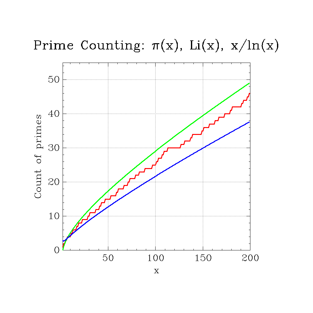
3.1.12 Prime Counting and Logarithmic Integral 
This plot compares the prime-counting staircase \pi(x) with smooth approximations such as Li(x) and x/\log x.
;;; ex-graph-riemann-stairs.scm — Prime-counting function and the logarithmic integral
;;; π(x) = number of primes ≤ x  (the prime-counting staircase)
;;; Li(x) = ∫₂ˣ dt/ln(t)       (the logarithmic integral)
;;; The Prime Number Theorem states π(x) ~ Li(x) ~ x/ln(x) as x → ∞.
;;; Also plots x/ln(x) to show Li(x) is a much better approximation.
;;; Uses symbols on π(x) to show discrete jumps at each prime.

(use-modules (srfi srfi-1)
             (plotutils graph))

(define (prime? n)
  (cond
   ((<= n 1) #f)
   ((= n 2) #t)
   ((even? n) #f)
   (else
    (let loop ((d 3))
      (cond
       ((> (* d d) n) #t)
       ((zero? (remainder n d)) #f)
       (else (loop (+ d 2))))))))

(define (pi-count x)
  "Count primes up to x."
  (let loop ((n 2) (count 0))
    (if (> n (inexact->exact (floor x)))
        count
        (loop (+ n 1) (if (prime? n) (+ count 1) count)))))

(define (integrate-simpson f a b n)
  (let* ((h (/ (- b a) n))
         (sum (+ (f a) (f b))))
    (let loop ((i 1) (s sum))
      (if (>= i n)
          (* (/ h 3.0) s)
          (let* ((xv (+ a (* i h)))
                 (w (if (even? i) 2.0 4.0)))
            (loop (+ i 1) (+ s (* w (f xv)))))))))

(define (li x)
  "Logarithmic integral Li(x) = ∫₂ˣ dt/ln(t)."
  (if (<= x 2.0) 0.0
      (integrate-simpson (lambda (t) (/ 1.0 (log t)))
                         2.0 x 200)))

(define (output-format-from-filename path)
  (let loop ((i (- (string-length path) 1)))
    (cond
     ((< i 0) "svg")
     ((char=? (string-ref path i) #\.)
      (let ((ext (string-downcase (substring path (+ i 1) (string-length path)))))
        (if (string=? ext "eps") "ps" ext)))
     (else (loop (- i 1))))))

(define (main args)
  (let* ((output-file (if (> (length args) 1) (cadr args) "graph-prime-counting.svg"))
         (output-format (output-format-from-filename output-file))
         ;; Staircase π(x) sampled at integers from 2 to 200
         (xmax 200)
         (integers (iota (- xmax 1) 2))
         (xs-pi (map exact->inexact integers))
         (ys-pi (map (lambda (n) (exact->inexact (pi-count n))) integers))

         ;; Li(x) as smooth curve
         (n 300)
         (step (/ (- xmax 2.0) n))
         (xs-li (iota n 2.0 step))
         (ys-li (map li xs-li))

         ;; x/ln(x) as comparison
         (ys-xlogx (map (lambda (x) (/ x (log x))) xs-li)))
    (with-output-to-file output-file
      (lambda ()
        (graph (merge xs-pi xs-li xs-li)
               (merge ys-pi ys-li ys-xlogx)
               #:output-format output-format
               #:bitmap-size "1000x1000"
               #:top-label "Prime Counting: \\*p(x), Li(x), x/ln(x)"
               #:x-label "x"
               #:y-label "Count of primes"
               #:x-limits '(2.0 200.0)
               #:y-limits '(0.0 55.0)
               #:toggle-use-color #t
               #:grid-style 3
               #:line-width 0.003
               #:font-name "HersheySerif"))
      #:binary #t)))

(main (command-line))
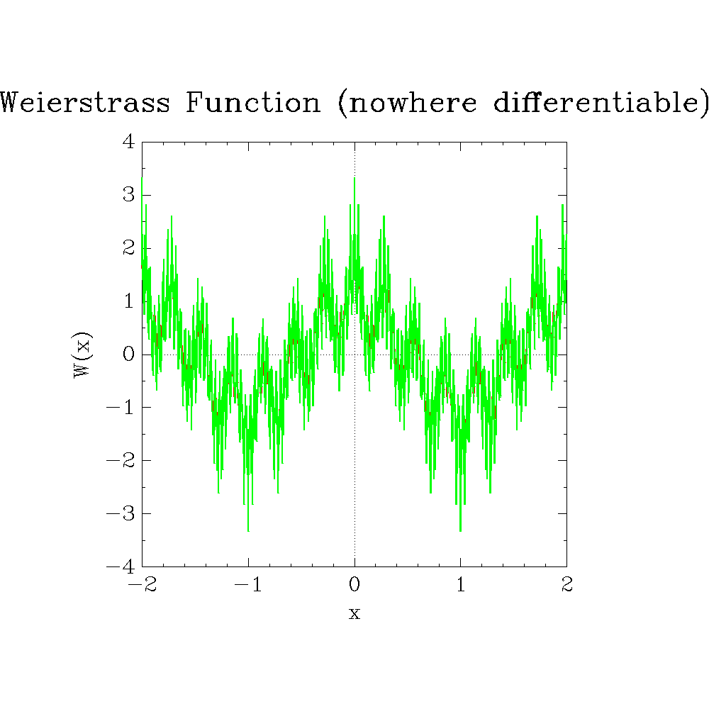
3.1.13 Weierstrass Function 
This plot draws a classic continuous but nowhere-differentiable Weierstrass function built from a cosine series.
;;; ex-graph-weierstrass.scm — Weierstrass function
;;; W(x) = Σ_{n=0}^{N} a^n · cos(b^n · π · x)
;;; With 0 < a < 1 and b a positive odd integer where a·b > 1+3π/2,
;;; this function is continuous everywhere but differentiable nowhere.
;;; A pathological example that shattered 19th-century intuitions about
;;; continuity implying differentiability.

(use-modules (srfi srfi-1)
             (plotutils graph))

(define pi (* 4.0 (atan 1.0)))

(define (weierstrass a b n-terms)
  "Return a procedure computing the Weierstrass function with N-TERMS terms."
  (lambda (x)
    (let loop ((n 0) (acc 0.0))
      (if (> n n-terms)
          acc
          (loop (+ n 1)
                (+ acc (* (expt a n) (cos (* (expt b n) pi x)))))))))

(define (output-format-from-filename path)
  (let loop ((i (- (string-length path) 1)))
    (cond
     ((< i 0) "svg")
     ((char=? (string-ref path i) #\.)
      (let ((ext (string-downcase (substring path (+ i 1) (string-length path)))))
        (if (string=? ext "eps") "ps" ext)))
     (else (loop (- i 1))))))

(define (main args)
  (let* ((output-file (if (> (length args) 1) (cadr args) "graph-weierstrass.svg"))
         (output-format (output-format-from-filename output-file))
         (n 2000)
         (xmin -2.0)
         (xmax 2.0)
         (step (/ (- xmax xmin) n))
         (xs (iota n xmin step))
         ;; Classic parameters: a=0.5, b=7
         (y1 (map (weierstrass 0.5 7 40) xs))
         ;; More jagged: a=0.7, b=7
         (y2 (map (weierstrass 0.7 7 30) xs)))
    (with-output-to-file output-file
      (lambda ()
        (graph (merge xs xs)
               (merge y1 y2)
               #:output-format output-format
               #:bitmap-size "1000x1000"
               #:top-label "Weierstrass Function (nowhere differentiable)"
               #:x-label "x"
               #:y-label "W(x)"
               #:x-limits '(-2.0 2.0)
               #:toggle-use-color #t
               #:grid-style 2
               #:line-width 0.002
               #:font-name "HersheySerif"))
      #:binary #t)))

(main (command-line))
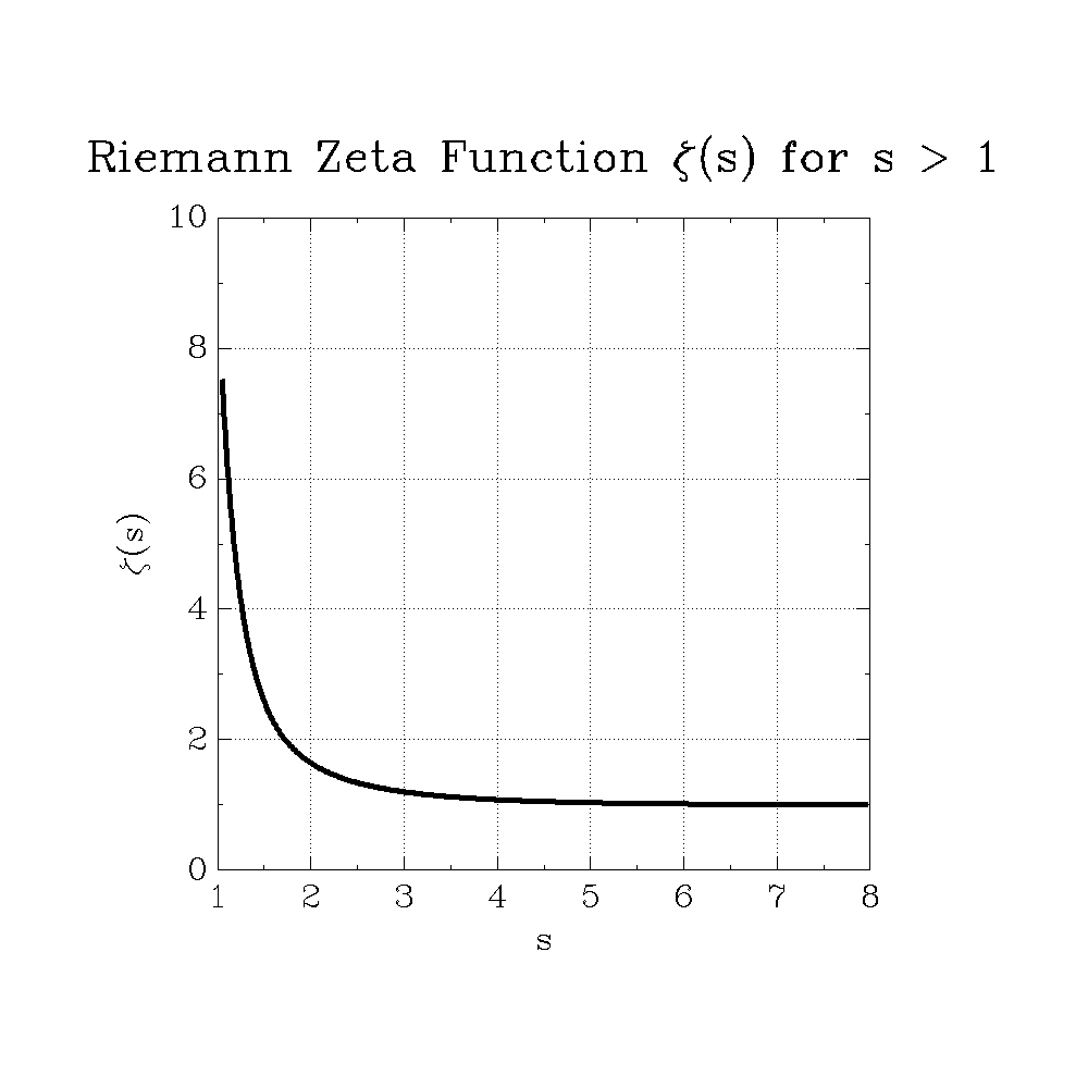
3.1.14 Riemann Zeta on the Real Line 
This plot shows numerical behavior of zeta(s) for real s > 1, including the blow-up near the pole at s=1.
;;; ex-graph-zeta.scm — The Riemann Zeta function on the real line
;;; Computes ζ(s) = Σ 1/n^s for s > 1 via partial sums, showing the
;;; pole at s=1 and decay toward 1 as s → ∞.  A central object in
;;; analytic number theory linking primes to complex analysis.

(use-modules (srfi srfi-1)
             (plotutils graph))

(define (zeta-partial s terms)
  "Approximate ζ(s) by summing the first TERMS terms of 1/n^s."
  (let loop ((n 1) (acc 0.0))
    (if (> n terms)
        acc
        (loop (+ n 1) (+ acc (/ 1.0 (expt n s)))))))

(define (output-format-from-filename path)
  (let loop ((i (- (string-length path) 1)))
    (cond
     ((< i 0) "svg")
     ((char=? (string-ref path i) #\.)
      (let ((ext (string-downcase (substring path (+ i 1) (string-length path)))))
        (if (string=? ext "eps") "ps" ext)))
     (else (loop (- i 1))))))

(define (main args)
  (let* ((output-file (if (> (length args) 1) (cadr args) "graph-zeta.svg"))
         (output-format (output-format-from-filename output-file))
         (n 400)
         (smin 1.05)
         (smax 8.0)
         (step (/ (- smax smin) n))
         (xs (iota n smin step))
         (ys (map (lambda (s) (zeta-partial s 5000)) xs)))
    (with-output-to-file output-file
      (lambda ()
        (graph xs ys
               #:output-format output-format
               #:bitmap-size "1000x1000"
               #:top-label "Riemann Zeta Function \\*z(s) for s > 1"
               #:x-label "s"
               #:y-label "\\*z(s)"
               #:x-limits '(1.0 8.0)
               #:y-limits '(0.0 10.0)
               #:grid-style 3
               #:line-width 0.005
               #:font-name "HersheySerif"))
      #:binary #t)))

(main (command-line))
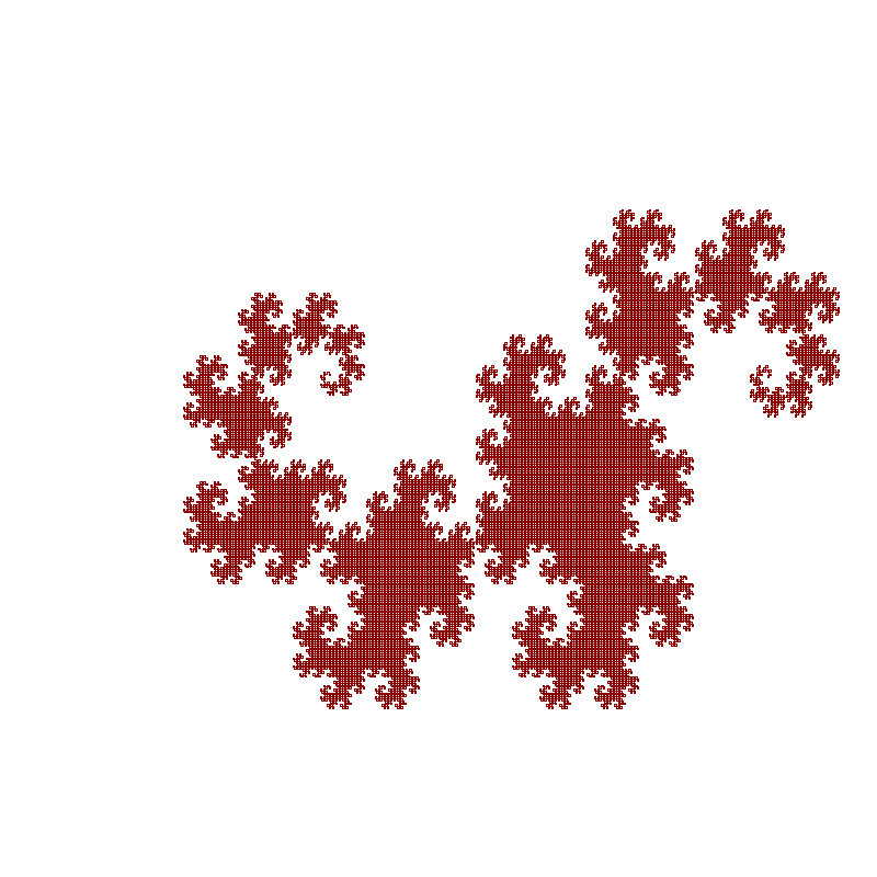
3.1.15 Dragon Curve 
This plot draws the Heighway dragon, a recursive fractal related to the paper-folding sequence.
;;; ex-plot-dragon-curve.scm — The Dragon Curve (Heighway Dragon)
;;; Discovered by physicist John Heighway and described by Martin Gardner,
;;; the dragon curve is a self-similar fractal.  It can be generated by
;;; repeatedly folding a strip of paper in half.  Its boundary is a fractal
;;; with Hausdorff dimension 2 (it is space-filling in the limit).
;;; The unfolding sequence follows the Regular Paper Folding Sequence.

(use-modules (plotutils plot))

(define pi (* 4.0 (atan 1.0)))

(define *plotter* #f)
(define *angle* 0.0)
(define *x* 0.0)
(define *y* 0.0)

(define (turtle-forward! dist)
  (let ((nx (+ *x* (* dist (cos (* *angle* (/ pi 180.0))))))
        (ny (+ *y* (* dist (sin (* *angle* (/ pi 180.0)))))))
    (cont! *plotter* nx ny)
    (set! *x* nx)
    (set! *y* ny)))

(define (turtle-left! degrees)
  (set! *angle* (+ *angle* degrees)))

(define (turtle-right! degrees)
  (set! *angle* (- *angle* degrees)))

(define (dragon-left depth length)
  "Draw dragon curve turning left at this level."
  (if (= depth 0)
      (turtle-forward! length)
      (begin
        (dragon-left (- depth 1) (/ length 1.41421356))
        (turtle-left! 90)
        (dragon-right (- depth 1) (/ length 1.41421356)))))

(define (dragon-right depth length)
  "Draw dragon curve turning right at this level."
  (if (= depth 0)
      (turtle-forward! length)
      (begin
        (dragon-left (- depth 1) (/ length 1.41421356))
        (turtle-right! 90)
        (dragon-right (- depth 1) (/ length 1.41421356)))))

(define (output-format-from-filename path)
  (let loop ((i (- (string-length path) 1)))
    (cond
     ((< i 0) "svg")
     ((char=? (string-ref path i) #\.)
      (let ((ext (string-downcase (substring path (+ i 1) (string-length path)))))
        (if (string=? ext "eps") "ps" ext)))
     (else (loop (- i 1))))))

(define (main args)
  (let* ((output-file (if (> (length args) 1) (cadr args) "plot-dragon-curve.svg"))
         (output-format (output-format-from-filename output-file))
         (fp (open-output-file output-file #:binary #t))
         (param (newplparams)))
    (setplparam! param "BITMAPSIZE" "800x800")
    (let ((plotter (newpl output-format fp (current-error-port) param)))
      (set! *plotter* plotter)
      (openpl! plotter)
      (space! plotter -100.0 -200.0 700.0 500.0)
      (linewidth! plotter 0.3)
      (erase! plotter)
      (pencolorname! plotter "dark red")

      (set! *x* 200.0)
      (set! *y* 200.0)
      (set! *angle* 0.0)
      (move! plotter *x* *y*)

      (dragon-left 16 400.0)

      (closepl! plotter)
      (close fp))))

(main (command-line))
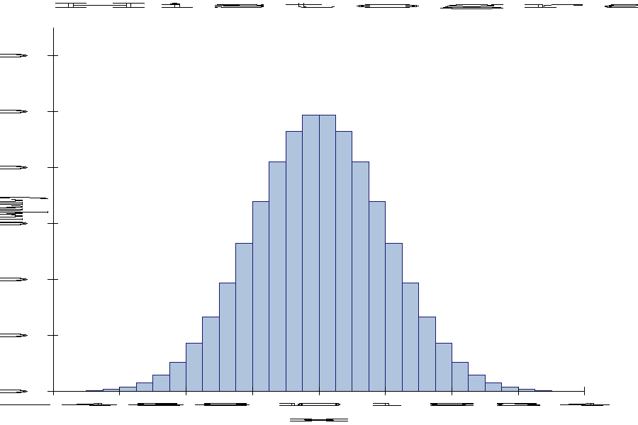
3.1.16 Gaussian Histogram 
This plot uses drawing primitives to render a histogram-like view of a Gaussian distribution with filled bars, axes, and labels.
;;; ex-plot-gaussian-histogram.scm — Gaussian histogram with filled bins
;;; Uses (plotutils plot) primitives to draw a histogram of a normal PDF
;;; with fixed bin width 0.25, including axes, ticks, labels, and title.

(use-modules (plotutils plot)
             (srfi srfi-1)
             (ice-9 format))

(define pi (* 4.0 (atan 1.0)))

(define (gaussian-pdf x mu sigma)
  (/ (exp (- (/ (* (- x mu) (- x mu)) (* 2.0 sigma sigma))))
     (* sigma (sqrt (* 2.0 pi)))))

(define (frange start stop step)
  "Create a numeric range [start, stop) with uniform step."
  (let loop ((x start) (acc '()))
    (if (>= x stop)
        (reverse acc)
        (loop (+ x step) (cons x acc)))))

(define (draw-histogram-bars! plotter bins bin-width mu sigma sample-size)
  "Draw filled histogram bars using Gaussian expected bin mass."
  (fillcolorname! plotter "lightsteelblue")
  (pencolorname! plotter "midnightblue")
  (filltype! plotter 1)
  (linewidth! plotter 0.08)
  (for-each
   (lambda (left)
     (let* ((right (+ left bin-width))
            (center (+ left (/ bin-width 2.0)))
            ;; Approximate bin count via midpoint rule.
            (height (* sample-size bin-width (gaussian-pdf center mu sigma))))
       (box! plotter left 0.0 right height)))
   bins)
  (filltype! plotter 0))

(define (draw-axes! plotter x-min x-max y-max)
  "Draw x/y axes with tick marks and numeric labels."
  (pencolorname! plotter "black")
  (linewidth! plotter 0.12)

  ;; Axes lines
  (line! plotter x-min 0.0 x-max 0.0)
  (line! plotter x-min 0.0 x-min y-max)

  ;; Tick styling text
  (fontname! plotter "HersheySerif")
  (fontsize! plotter 1.5)

  ;; X-axis ticks and labels at integer points
  (for-each
   (lambda (x)
     (line! plotter x -1.5 x 1.5)
     (move! plotter x -4.0)
     (alabel! plotter 'c 't (format #f "~a" (inexact->exact (round x)))))
   (frange -4.0 4.1 1.0))

  ;; Y-axis ticks and labels every 20 units
  (for-each
   (lambda (y)
     (line! plotter (- x-min 0.08) y (+ x-min 0.08) y)
     (move! plotter (- x-min 0.25) y)
     (alabel! plotter 'r 'c (format #f "~a" (inexact->exact (round y)))))
   (frange 0.0 (+ y-max 0.1) 20.0)))

(define (draw-labels! plotter x-min x-max y-max)
  "Draw axis labels and figure title."
  (pencolorname! plotter "black")

  ;; Title
  (fontname! plotter "HersheySerif")
  (fontsize! plotter 2.2)
  (move! plotter (/ (+ x-min x-max) 2.0) (+ y-max 8.0))
  (alabel! plotter 'c 'c "Gaussian Distribution Histogram (bin width = 0.25)")

  ;; X-axis label
  (fontsize! plotter 1.8)
  (move! plotter (/ (+ x-min x-max) 2.0) -10.0)
  (alabel! plotter 'c 'c "x")

  ;; Y-axis label (rotated)
  (textangle! plotter 90.0)
  (move! plotter (- x-min 0.95) (/ y-max 2.0))
  (alabel! plotter 'c 'c "Frequency")
  (textangle! plotter 0.0))

(define (output-format-from-filename path)
  (let loop ((i (- (string-length path) 1)))
    (cond
     ((< i 0) "svg")
     ((char=? (string-ref path i) #\.)
      (let ((ext (string-downcase (substring path (+ i 1) (string-length path)))))
        (if (string=? ext "eps") "ps" ext)))
     (else (loop (- i 1))))))

(define (main args)
  (let* ((output-file (if (> (length args) 1) (cadr args) "plot-gaussian-histogram.svg"))
         (output-format (output-format-from-filename output-file))
         (fp (open-output-file output-file #:binary #t))
         (param (newplparams))
         (bin-width 0.25)
         (x-min -4.0)
         (x-max 4.0)
         (y-max 130.0)
         (mu 0.0)
         (sigma 1.0)
         (sample-size 1000.0)
         (bins (frange x-min x-max bin-width)))

    (setplparam! param "BITMAPSIZE" "900x600")

    (let ((plotter (newpl output-format fp (current-error-port) param)))
      (openpl! plotter)

      ;; Leave margins for axis labels and title.
      (space! plotter -4.8 -12.0 4.8 140.0)
      (erase! plotter)
      (bgcolorname! plotter "white")

      (draw-histogram-bars! plotter bins bin-width mu sigma sample-size)
      (draw-axes! plotter x-min x-max y-max)
      (draw-labels! plotter x-min x-max y-max)

      (closepl! plotter)
      (close fp))))

(main (command-line))
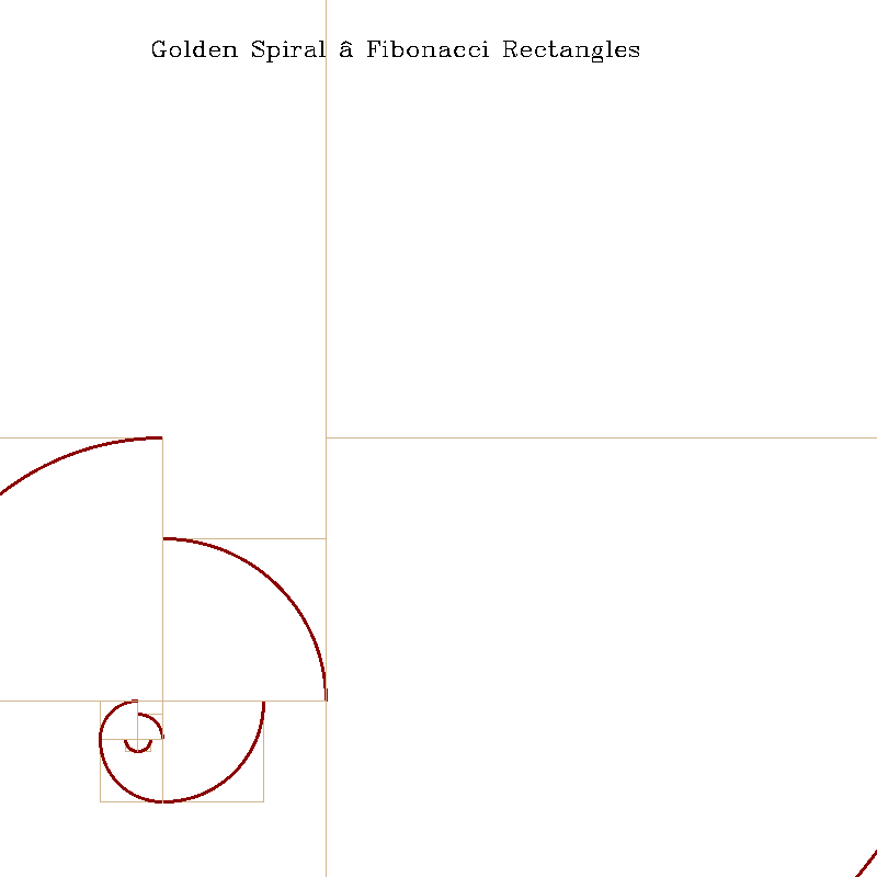
3.1.17 Golden Spiral 
This plot constructs a golden spiral approximation from Fibonacci-sized squares and quarter-circle arcs.
;;; ex-plot-golden-spiral.scm — Golden Spiral constructed from Fibonacci arcs
;;; The golden spiral is a logarithmic spiral whose growth factor is ϕ,
;;; the golden ratio (1+√5)/2 ≈ 1.618.  Here it is approximated by
;;; quarter-circle arcs inscribed in squares whose side lengths follow
;;; the Fibonacci sequence: 1, 1, 2, 3, 5, 8, 13, 21, ...
;;; Also draws the Fibonacci rectangle tiling underneath.
;;; This construction connects number theory (Fibonacci/Lucas numbers),
;;; geometry (logarithmic spirals), and phyllotaxis in nature.

(use-modules (plotutils plot))

(define (fibonacci-list n)
  "Return the first N Fibonacci numbers starting from 1, 1."
  (let loop ((i 2) (a 1) (b 1) (acc (list 1 1)))
    (if (>= i n) (reverse acc)
        (let ((c (+ a b)))
          (loop (+ i 1) b c (cons c acc))))))

(define (output-format-from-filename path)
  (let loop ((i (- (string-length path) 1)))
    (cond
     ((< i 0) "svg")
     ((char=? (string-ref path i) #\.)
      (let ((ext (string-downcase (substring path (+ i 1) (string-length path)))))
        (if (string=? ext "eps") "ps" ext)))
     (else (loop (- i 1))))))

(define (main args)
  (let* ((output-file (if (> (length args) 1) (cadr args) "plot-golden-spiral.svg"))
         (output-format (output-format-from-filename output-file))
         (fp (open-output-file output-file #:binary #t))
         (param (newplparams)))
    (setplparam! param "BITMAPSIZE" "800x800")
    (let ((plotter (newpl output-format fp (current-error-port) param)))
      (openpl! plotter)
      (space! plotter -10.0 -10.0 60.0 60.0)
      (erase! plotter)

      (let* ((fibs (fibonacci-list 11))
             (scale 1.0))

        ;; We'll track the corner of each square and direction of growth.
        ;; Directions cycle: right, up, left, down (quadrant rotation)
        ;; Start at origin, first two 1×1 squares.
        (let loop ((remaining fibs)
                   (cx 0.0) (cy 0.0)  ; current square corner (lower-left)
                   (dir 0))            ; 0=right, 1=up, 2=left, 3=down
          (when (pair? remaining)
            (let* ((s (* (car remaining) scale)) ; side length
                   ;; Compute the four corners of this square based on direction
                   ;; The arc sweeps a quarter circle from one edge to the next
                   )
              ;; Draw the square
              (pencolorname! plotter "tan")
              (linewidth! plotter 0.1)
              (box! plotter cx cy (+ cx s) (+ cy s))

              ;; Draw the quarter-circle arc inscribed in this square
              (pencolorname! plotter "dark red")
              (linewidth! plotter 0.3)
              (let* ((qdir (modulo dir 4))
                     ;; The arc center depends on which corner of the square
                     ;; dir=0: arc centered at upper-right, from upper-left to lower-right
                     ;; dir=1: arc centered at upper-left, from lower-left to upper-right
                     ;; dir=2: arc centered at lower-left, from lower-right to upper-left
                     ;; dir=3: arc centered at lower-right, from upper-right to lower-left
                     (acx (cond ((= qdir 0) (+ cx s)) ((= qdir 1) cx)
                                ((= qdir 2) cx)       ((= qdir 3) (+ cx s))))
                     (acy (cond ((= qdir 0) (+ cy s)) ((= qdir 1) (+ cy s))
                                ((= qdir 2) cy)       ((= qdir 3) cy)))
                     (ax0 (cond ((= qdir 0) cx)       ((= qdir 1) cx)
                                ((= qdir 2) (+ cx s)) ((= qdir 3) (+ cx s))))
                     (ay0 (cond ((= qdir 0) (+ cy s)) ((= qdir 1) cy)
                                ((= qdir 2) cy)       ((= qdir 3) (+ cy s))))
                     (ax1 (cond ((= qdir 0) (+ cx s)) ((= qdir 1) (+ cx s))
                                ((= qdir 2) cx)       ((= qdir 3) cx)))
                     (ay1 (cond ((= qdir 0) cy)       ((= qdir 1) (+ cy s))
                                ((= qdir 2) (+ cy s)) ((= qdir 3) cy))))
                (arc! plotter acx acy ax0 ay0 ax1 ay1))

              ;; Compute next square's lower-left corner
              (let* ((qdir (modulo dir 4))
                     (ncx (cond ((= qdir 0) (+ cx s)) ((= qdir 1) cx)
                                ((= qdir 2) (- cx (car (if (pair? (cdr remaining))
                                                            (cdr remaining) (list s)))))
                                ((= qdir 3) cx)))
                     (ncy (cond ((= qdir 0) cy)       ((= qdir 1) (+ cy s))
                                ((= qdir 2) cy)
                                ((= qdir 3) (- cy (car (if (pair? (cdr remaining))
                                                            (cdr remaining) (list s))))))))
                (loop (cdr remaining) ncx ncy (+ dir 1)))))))

      ;; Title
      (pencolorname! plotter "black")
      (move! plotter 2.0 56.0)
      (fontname! plotter "HersheySerif")
      (fontsize! plotter 2.0)
      (alabel! plotter 'l 'c "Golden Spiral — Fibonacci Rectangles")

      (closepl! plotter)
      (close fp))))

(main (command-line))
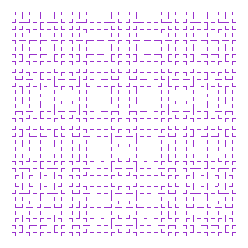
3.1.18 Hilbert Curve 
This plot draws a Hilbert space-filling curve, a recursive path that visits each cell of a grid in a locality-preserving order.
;;; ex-plot-hilbert-curve.scm — Hilbert space-filling curve
;;; The Hilbert curve is a continuous fractal space-filling curve
;;; first described by David Hilbert in 1891.  At each level of
;;; recursion it visits every cell of a 2^n × 2^n grid exactly once.
;;; In the limit, it maps the unit interval [0,1] surjectively onto the
;;; unit square [0,1]², providing a continuous mapping from 1D to 2D.

(use-modules (plotutils plot))

(define pi (* 4.0 (atan 1.0)))

(define *plotter* #f)
(define *angle* 0.0)
(define *x* 0.0)
(define *y* 0.0)

(define (turtle-forward! dist)
  (let ((nx (+ *x* (* dist (cos (* *angle* (/ pi 180.0))))))
        (ny (+ *y* (* dist (sin (* *angle* (/ pi 180.0)))))))
    (cont! *plotter* nx ny)
    (set! *x* nx)
    (set! *y* ny)))

(define (turtle-left! degrees)
  (set! *angle* (+ *angle* degrees)))

(define (turtle-right! degrees)
  (set! *angle* (- *angle* degrees)))

(define (hilbert level size parity)
  "Draw a Hilbert curve of given level. PARITY is +1 or -1."
  (when (> level 0)
    (turtle-left! (* parity 90))
    (hilbert (- level 1) size (- parity))
    (turtle-forward! size)
    (turtle-right! (* parity 90))
    (hilbert (- level 1) size parity)
    (turtle-forward! size)
    (hilbert (- level 1) size parity)
    (turtle-right! (* parity 90))
    (turtle-forward! size)
    (hilbert (- level 1) size (- parity))
    (turtle-left! (* parity 90))))

(define (output-format-from-filename path)
  (let loop ((i (- (string-length path) 1)))
    (cond
     ((< i 0) "svg")
     ((char=? (string-ref path i) #\.)
      (let ((ext (string-downcase (substring path (+ i 1) (string-length path)))))
        (if (string=? ext "eps") "ps" ext)))
     (else (loop (- i 1))))))

(define (main args)
  (let* ((output-file (if (> (length args) 1) (cadr args) "plot-hilbert-curve.svg"))
         (output-format (output-format-from-filename output-file))
         (fp (open-output-file output-file #:binary #t))
         (param (newplparams)))
    (setplparam! param "BITMAPSIZE" "800x800")
    (let* ((plotter (newpl output-format fp (current-error-port) param))
           (order 6)
           (cells (- (expt 2 order) 1))
           (step (/ 760.0 cells)))
      (set! *plotter* plotter)
      (openpl! plotter)
      (space! plotter -20.0 -20.0 820.0 820.0)
      (linewidth! plotter 0.5)
      (erase! plotter)
      (pencolorname! plotter "dark orchid")

      ;; Start at lower left
      (set! *x* 20.0)
      (set! *y* 20.0)
      (set! *angle* 0.0)
      (move! plotter *x* *y*)

      (hilbert order step 1)

      (closepl! plotter)
      (close fp))))

(main (command-line))
3.1.19 Koch Snowflake 
This plot draws the Koch snowflake, a fractal curve with infinite perimeter but finite enclosed area.

;;; ex-plot-koch-snowflake.scm — Koch Snowflake fractal
;;; The Koch snowflake is constructed by starting with an equilateral
;;; triangle and recursively replacing the middle third of each edge
;;; with two sides of a smaller equilateral triangle.  Its perimeter
;;; is infinite while enclosing finite area.  Hausdorff dimension = log4/log3 ≈ 1.2619.

(use-modules (plotutils plot))

(define pi (* 4.0 (atan 1.0)))

(define *plotter* #f)
(define *angle* 0.0)
(define *x* 0.0)
(define *y* 0.0)

(define (turtle-forward! dist)
  (let ((nx (+ *x* (* dist (cos (* *angle* (/ pi 180.0))))))
        (ny (+ *y* (* dist (sin (* *angle* (/ pi 180.0)))))))
    (cont! *plotter* nx ny)
    (set! *x* nx)
    (set! *y* ny)))

(define (turtle-left! degrees)
  (set! *angle* (+ *angle* degrees)))

(define (turtle-right! degrees)
  (set! *angle* (- *angle* degrees)))

(define (koch-segment length depth)
  "Draw one Koch curve segment of given length at given recursion depth."
  (if (= depth 0)
      (turtle-forward! length)
      (begin
        (koch-segment (/ length 3.0) (- depth 1))
        (turtle-left! 60)
        (koch-segment (/ length 3.0) (- depth 1))
        (turtle-right! 120)
        (koch-segment (/ length 3.0) (- depth 1))
        (turtle-left! 60)
        (koch-segment (/ length 3.0) (- depth 1)))))

(define (koch-snowflake side depth)
  "Draw a complete Koch snowflake (3 Koch curve segments)."
  (koch-segment side depth)
  (turtle-right! 120)
  (koch-segment side depth)
  (turtle-right! 120)
  (koch-segment side depth))

(define (output-format-from-filename path)
  (let loop ((i (- (string-length path) 1)))
    (cond
     ((< i 0) "svg")
     ((char=? (string-ref path i) #\.)
      (let ((ext (string-downcase (substring path (+ i 1) (string-length path)))))
        (if (string=? ext "eps") "ps" ext)))
     (else (loop (- i 1))))))

(define (main args)
  (let* ((output-file (if (> (length args) 1) (cadr args) "plot-koch-snowflake.svg"))
         (output-format (output-format-from-filename output-file))
         (fp (open-output-file output-file #:binary #t))
         (param (newplparams)))
    (setplparam! param "BITMAPSIZE" "800x800")
    (let ((plotter (newpl output-format fp (current-error-port) param)))
      (set! *plotter* plotter)
      (openpl! plotter)
      (space! plotter -50.0 -50.0 850.0 850.0)
      (linewidth! plotter 0.5)
      (erase! plotter)
      (bgcolorname! plotter "white")
      (pencolorname! plotter "navy")

      ;; Position at top-left of the snowflake
      (set! *x* 100.0)
      (set! *y* 650.0)
      (set! *angle* -60.0)
      (move! plotter *x* *y*)

      (koch-snowflake 600.0 5)

      (closepl! plotter)
      (close fp))))

(main (command-line))
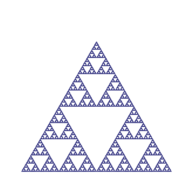
3.1.20 Sierpinski Triangle 
This plot draws the Sierpinski triangle (gasket), a canonical self-similar fractal obtained by recursive subdivision.
;;; ex-plot-sierpinski-triangle.scm — Sierpiński Triangle
;;; The Sierpiński triangle (Sierpiński gasket) is a fractal attractor
;;; described by Wacław Sierpiński in 1915.  It is formed by recursively
;;; subdividing an equilateral triangle into four smaller equilateral
;;; triangles and removing the central one.  It has Hausdorff dimension
;;; log(3)/log(2) ≈ 1.585.  It also arises in Pascal's triangle
;;; (cells with odd binomial coefficients) and in the Chaos Game.

(use-modules (plotutils plot))

(define *plotter* #f)

(define (draw-filled-triangle! x1 y1 x2 y2 x3 y3 color)
  "Draw a filled triangle with the given vertices."
  (pencolorname! *plotter* color)
  (fillcolorname! *plotter* color)
  (filltype! *plotter* 1)
  (move! *plotter* x1 y1)
  (cont! *plotter* x2 y2)
  (cont! *plotter* x3 y3)
  (cont! *plotter* x1 y1)
  (endpath! *plotter*)
  (filltype! *plotter* 0))

(define (sierpinski depth x1 y1 x2 y2 x3 y3)
  "Recursively draw the Sierpiński triangle."
  (if (= depth 0)
      (draw-filled-triangle! x1 y1 x2 y2 x3 y3 "midnight blue")
      (let ((mx12 (/ (+ x1 x2) 2.0)) (my12 (/ (+ y1 y2) 2.0))
            (mx23 (/ (+ x2 x3) 2.0)) (my23 (/ (+ y2 y3) 2.0))
            (mx13 (/ (+ x1 x3) 2.0)) (my13 (/ (+ y1 y3) 2.0)))
        ;; Bottom-left triangle
        (sierpinski (- depth 1) x1 y1 mx12 my12 mx13 my13)
        ;; Bottom-right triangle
        (sierpinski (- depth 1) mx12 my12 x2 y2 mx23 my23)
        ;; Top triangle
        (sierpinski (- depth 1) mx13 my13 mx23 my23 x3 y3))))

(define (output-format-from-filename path)
  (let loop ((i (- (string-length path) 1)))
    (cond
     ((< i 0) "svg")
     ((char=? (string-ref path i) #\.)
      (let ((ext (string-downcase (substring path (+ i 1) (string-length path)))))
        (if (string=? ext "eps") "ps" ext)))
     (else (loop (- i 1))))))

(define (main args)
  (let* ((output-file (if (> (length args) 1) (cadr args) "plot-sierpinski-triangle.svg"))
         (output-format (output-format-from-filename output-file))
         (fp (open-output-file output-file #:binary #t))
         (param (newplparams)))
    (setplparam! param "BITMAPSIZE" "800x800")
    (let ((plotter (newpl output-format fp (current-error-port) param)))
      (set! *plotter* plotter)
      (openpl! plotter)
      (space! plotter -50.0 -50.0 850.0 850.0)
      (linewidth! plotter 0.2)
      (erase! plotter)

      ;; Equilateral triangle vertices
      (let* ((side 700.0)
             (height (* side (/ (sqrt 3.0) 2.0)))
             (x1 50.0) (y1 50.0)
             (x2 (+ x1 side)) (y2 50.0)
             (x3 (+ x1 (/ side 2.0))) (y3 (+ 50.0 height)))
        (sierpinski 8 x1 y1 x2 y2 x3 y3))

      (closepl! plotter)
      (close fp))))

(main (command-line))
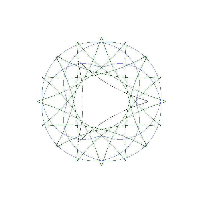
3.1.21 Spirograph Curves 
This plot draws hypotrochoid and epitrochoid-style roulette curves, popularized by mechanical spirograph toys.
;;; ex-plot-spirograph.scm — Spirograph (Hypotrochoid and Epitrochoid) curves
;;; A hypotrochoid is traced by a point attached to a circle of radius r
;;; rolling inside a fixed circle of radius R:
;;;   x(t) = (R−r)cos(t) + d·cos((R−r)t/r)
;;;   y(t) = (R−r)sin(t) − d·sin((R−r)t/r)
;;; An epitrochoid rolls outside:
;;;   x(t) = (R+r)cos(t) − d·cos((R+r)t/r)
;;;   y(t) = (R+r)sin(t) − d·sin((R+r)t/r)
;;; These curves belong to the family of roulettes studied since
;;; Dürer (1525) and were popularized by the Spirograph toy (1965).

(use-modules (plotutils plot))

(define pi (* 4.0 (atan 1.0)))

(define (draw-hypotrochoid! plotter R r d n-steps color)
  "Draw a hypotrochoid on plotter with given parameters."
  (pencolorname! plotter color)
  (let* ((dt (/ (* 2.0 pi) n-steps))
         (x0 (+ (- R r) d))
         (y0 0.0))
    (move! plotter x0 y0)
    (let loop ((i 1))
      (if (<= i (* n-steps 10))  ; go around enough times for closure
          (let* ((t (* i dt))
                 (x (+ (* (- R r) (cos t))
                        (* d (cos (* (/ (- R r) r) t)))))
                 (y (- (* (- R r) (sin t))
                        (* d (sin (* (/ (- R r) r) t))))))
            ;; Stop if we've returned very close to start after at least one loop
            (if (and (> i n-steps)
                     (< (+ (* (- x x0) (- x x0)) (* (- y y0) (- y y0))) 0.01))
                (cont! plotter x0 y0)
                (begin
                  (cont! plotter x y)
                  (loop (+ i 1)))))))))

(define (draw-epitrochoid! plotter R r d n-steps color)
  "Draw an epitrochoid on plotter with given parameters."
  (pencolorname! plotter color)
  (let* ((dt (/ (* 2.0 pi) n-steps))
         (x0 (- (+ R r) d))
         (y0 0.0))
    (move! plotter x0 y0)
    (let loop ((i 1))
      (if (<= i (* n-steps 12))
          (let* ((t (* i dt))
                 (x (- (* (+ R r) (cos t))
                        (* d (cos (* (/ (+ R r) r) t)))))
                 (y (- (* (+ R r) (sin t))
                        (* d (sin (* (/ (+ R r) r) t))))))
            (if (and (> i n-steps)
                     (< (+ (* (- x x0) (- x x0)) (* (- y y0) (- y y0))) 0.01))
                (cont! plotter x0 y0)
                (begin
                  (cont! plotter x y)
                  (loop (+ i 1)))))))))

(define (output-format-from-filename path)
  (let loop ((i (- (string-length path) 1)))
    (cond
     ((< i 0) "svg")
     ((char=? (string-ref path i) #\.)
      (let ((ext (string-downcase (substring path (+ i 1) (string-length path)))))
        (if (string=? ext "eps") "ps" ext)))
     (else (loop (- i 1))))))

(define (main args)
  (let* ((output-file (if (> (length args) 1) (cadr args) "plot-spirograph.svg"))
         (output-format (output-format-from-filename output-file))
         (fp (open-output-file output-file #:binary #t))
         (param (newplparams)))
    (setplparam! param "BITMAPSIZE" "800x800")
    (let ((plotter (newpl output-format fp (current-error-port) param)))
      (openpl! plotter)
      (space! plotter -220.0 -220.0 220.0 220.0)
      (linewidth! plotter 0.4)
      (erase! plotter)

      ;; Hypotrochoid #1: R=105, r=35, d=30  (a 3-lobed rose-like)
      (draw-hypotrochoid! plotter 105.0 35.0 30.0 2000 "crimson")

      ;; Hypotrochoid #2: R=144, r=45, d=40  (a rich multi-petal)
      (draw-hypotrochoid! plotter 144.0 45.0 40.0 2000 "dark green")

      ;; Epitrochoid: R=60, r=45, d=30
      (draw-epitrochoid! plotter 60.0 45.0 30.0 2000 "royal blue")

      (closepl! plotter)
      (close fp))))

(main (command-line))